 |
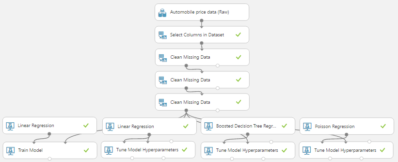
| Experiment So Far |
 |
| Automobile Price Data (Clean) 1 |
 |
| Automobile Price Data (Clean) 2 |
Poisson Regression is used to predict values that have a Poisson Distribution, i.e. counts within a given timeframe. For example, the number of customers that enter a store on a given day may follow a Poisson Distribution. Given that these values are counts, there are a couple of caveats. First, the counts cannot be negative. Second, the counts could theoretically extend to infinity. Finally, the counts must be Whole Numbers.
Just by looking at these three criteria, it may seem like Poisson Regression is theoretically appropriate for this data set. However, the issue comes when we consider the mathematical underpinning of the Poisson Distribution. Basically, the Poisson Distribution assumes that each entity being counted operates independently of the other entities. Back to our earlier example, we assume that each customer entering the store on a given day does so without considering whether the other customers will be going to the store on that day as well. Comparing this to our vehicle price data, that would be akin to saying that when a car is bought, each dollar independently decides whether it wants to jump out of the buyer's pocket and into the seller's hand. Obviously, this is a ludicrous notion. However, we're not theoretical purists and love bending rules (as long as they produce good results). For us, the true test comes from the validation portion of the experiment, which we'll cover in a later post. If you want to learn more about Poisson Regression, read this and this. Let's take a look at the parameters for this module.
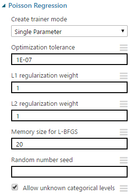 |
| Poisson Regression |
Without going into too much depth, the "L1 Regularization Weight" and "L2 Regularization Weight" parameters penalize complex models. If you want to learn more about Regularization, read this and this. As with "Optimization Tolerance", Azure ML will choose this value for us.
"Memory Size for L-BFGS" specifies the amount of memory allocated to the L-BFGS algorithm. We can't find much more information about what effect changing this value will have. Through some testing, we did find that this value had very little impact on our model, regardless of how large or small we made it (the minimum value we could provide is 1). However, if our data set had an extremely large number of columns, we may find that this parameter becomes more significant. Once again, we do not have to choose this value ourselves.
The "Random Number Seed" parameter allows us to create reproducible results for presentation/demonstration purposes. Oddly enough, we'd expect this value to play a role in the L-BFGS algorithm, but it doesn't seem to. We were unable to find any impact caused by changing this value.
Finally, we can choose to deselect "Allow Unknown Categorical Levels". When we train our model, we do so using a specific data set known as the training set. This allows the model to predict based on values it has seen before. For instance, our model has seen "Num of Doors" values of "two" and "four". So, what happens if we try to use the model to predict the price for a vehicle with a "Num of Doors" value of "three" or "five"? If we leave this option selected, then this new vehicle will have its "Num of Doors" value thrown into an "Unknown" category. This would mean that if we had a vehicle with three doors and another vehicle with five doors, they would both be thrown into the same "Num of Doors" category. To see exactly how this works, check out of our previous post, Regression Using Linear Regression (Ordinary Least Squares).
The options for the "Create Trainer Mode" parameter are "Single Parameter" and "Parameter Range". When we choose "Parameter Range", we instead supply a list of values for each parameter and the algorithm will build multiple models based on the lists. These multiple models must then be whittled down to a single model using the "Tune Model Hyperparameters" module. This can be really useful if we have a list of candidate models and want to be able to compare them quickly. However, we don't have a list of candidate models, but that actually makes "Tune Model Hyperparameters" more useful. We have no idea what the best set of parameters would be for this data. So, let's use it to choose our parameters for us.
 |
| Tune Model Hyperparameters |
 |
| Tune Model Hyperparameters (Visualization) |
On a side note, there is a display issue causing some values for the "Optimization Tolerance" parameter to display as 0 instead of whatever extremely small value they actually are. This is disappointing as it limits our ability to manually type these values into the "Poisson Regression" module. One of the outputs from the "Tune Model Hyperparameters" module is the Trained Best Model, whichever model appears at the top of list based on the metric we chose. This means that we can use this as an input into other modules like "Score Model". However, it does mean that we cannot use these parameters in conjunction with the "Cross Validate Model" module as that requires an Untrained Model as an input. Alas, this is not a huge deal because we see that "Optimization Tolerance" does not have a very large effect on the resulting model.
 |
| All Regression Models Complete |
Brad Llewellyn
Data Scientist
Valorem
@BreakingBI
www.linkedin.com/in/bradllewellyn
llewellyn.wb@gmail.com
No comments:
Post a Comment