Monday, March 20, 2017

Azure Machine Learning: Regression Using Linear Regression (Ordinary Least Squares)

Today, we're going to continue our walkthrough of Sample 4: Cross Validation for Regression: Auto Imports Dataset.  In the previous post, we walked through the initial data load and imputation phases of the experiment.
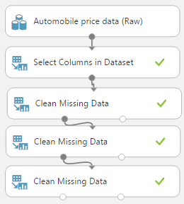
Initial Data Load and Imputation
Let's refresh our memory on the data set.
Automobile Price Data (Clean) 1

Automobile Price Data (Clean) 2
We can see that this data set contains a bunch of text and numeric data about each vehicle, as well as its price.  The goal of this experiment is to attempt to predict the price of the car based on these factors.  One way to do this is through a technique called Regression.  Basically, regression is a technique for predicting a numeric value (or set of values) based on a series of numeric inputs.

Now, some of you might be asking what happens to the non-numeric text data.  Turns out, they get converted into numeric variables using a technique called Indicator Variables (also known as Dummy Variables).  With this technique, every text field gets broken down into multiple binary (0/1) fields, each representing a single unique value from the original field.  For instance, the Num of Doors fields takes the values "two" and "four".  Therefore, the Indicator Variables for this field would be "Num of Doors = two" and "Num of Doors = four".  Each of these fields takes a value of 1 if the original field contains the value in question, and 0 if it doesn't.  To continue our example, a vehicle with "Num of Doors" = "two" would have a value of 1 in the "Num of Doors = two" field and a value of 0 in the "Num of Doors = four" field.
Indicator Variables Example
Things actually get a little more complicated when you are dealing with Unknown/NULL values.  The specific technique used varies based on the tool, but rarely has any effect.  We'll see how things works for Linear Regression later in this post.  As a side note, not all modules will automatically convert your fields to Indicator Variables.  In these cases, Azure ML has a module called Convert to Indicator Values that will do this for you.  If we need finer control over exactly how it accomplishes this, we could also use a SQL, R or Python script to handle it.  Let's move on to Linear Regression.

Earlier, we mentioned that Regression is a technique for predicting numeric values using other numeric values.  Linear Regression is a subset of Regression that creates a very specific type of model.  Let's say that we are trying to predict a value x by using values y and z.  A linear regression algorithm will create a model that looks like x = a*y + b*z + c, where a, b and c are called "coefficients", also known as "weights".  Now, this relationship looks linear from the coefficients' perspectives (meaning that there are no exponents, trigonometric functions, etc.).  However, if were to alter our data set so that z = y^2, then we would end up with the model x = a*y + b*y^2 + c.  This is LINEAR from the coefficients' perspectives, but is PARABOLIC from variables' perspectives.  This is one of the major reasons why Linear Regression is so popular.  It's very easy to build, train and comprehend, but is virtually limitless in the amount of relationships it can handle.  Let's take a look at the parameters.
Linear Regression (OLS)
We see that there are two options for "Solution Method".  The first, and most common, method is "Ordinary Least Squares" (OLS).  This method is the one most commonly taught because it has almost no parameters to tinker with.  We basically toss our data at it and it runs.  OLS is also very efficient because the entire algorithm is just a short series of linear algebra operations and only runs through the data once.  You can learn more about OLS here.

The second option for "Solution Method" is "Online Gradient Descent".  This method is substantially more complicated and will be covered in the next post.

Without going into too much depth, the "L2 Regularization Weight" parameter penalizes complex models.  Unfortunately, the "Tune Model Hyperparameters" module will not choose this value for us.  On the other hand, we tried a few values and did not find it to have any significant impact on our model.  If you want to learn more about Regularization, read this and this.

We can also choose "Include Intercept Term".  If we deselect this option, then our model will change from x = a*y + b*z + c to x = a*y + b*z.  This means that when all of our factors are 0, then our prediction would also be zero.  Honestly, we've never found a reason, in school or in practice, why we would ever want to deselect this option.  If you know of any, please let us know in the comments.

Next, we can choose a "Random Number Seed".  Most machine learning algorithms are random by nature.  That means their "starting point" matters.  Running the algorithm multiple times will produce different results.  However, the OLS algorithm is not random.  We tested and confirmed that this parameter has no impact on this algorithm.

Finally, we can choose to deselect "Allow Unknown Categorical Levels".  When we train our model, we do so using a specific data set known as the training set.  This allows the model to predict based on values it has seen before.  For instance, our model has seen "Num of Doors" values of "two" and "four".  So, what happens if we try to use the model to predict the price for a vehicle with a "Num of Doors" value of "three" or "five"?  If we leave this option selected, then this new vehicle will have its "Num of Doors" value thrown into an "Unknown" category.  This would mean that if we had a vehicle with three doors and another vehicle with five doors, they would both be thrown into the same "Num of Doors" category.  We'll see exactly how this works when we look at the indicator variables.

Now that we know understand the parameters behind the OLS module, let's look at the results of the "Train Model" module.
Train Model
Train Model (Visualization)


We can see that the visualization is made up of two sections, "Settings" and "Feature Weights".  The "Settings" section simply shows us what parameters we set in the module.  The "Feature Weights" section shows us all of the independent variables (everything except what we were trying to predict, which was Price) as well as their "Weight" or "Coefficient".  Positive weights mean that the value has a positive effect on price and Negative weights mean that the value has a negative effect on price.  Let's take a closer look at some of the different features.
Features
We can see that there are quite a few different features in this model.  We've pulled out a few and color coded them for clarity.  Let's start with "Bias".  Remember back to our model equation, x = a*y + b*z + c.  The "Bias" value corresponds to c in our equation.  This tells us that if all of our other factors were 0 (which is impossible for some of our factors), the price of our car would be -$6,008.57.  Obviously, this is a silly value.  Bias, also known as the intercept, is not generally a useful value by itself.  However, it does greatly improve the fit of our models and can be utilized by more advanced techniques.

Next, let's take a look at the features in Grey.  These are all numeric features.  We can tell because they don't have any underscores (_) or pound signs (#) in them.  We see that cars with an additional "Width" of 1, would also have an additional price of $600.89.  We can also see that vehicles will larger values of "Bore" and "Stroke" have lower prices.

Let's move on to the features in Blue.  These are the Indicator Variables we've mentioned a couple of time.  In our original data set, we included a feature called "body-style".  This feature had the values "convertible", "hardtop", "hatchback", "sedan" and "wagon".  Therefore, when the Linear Regression module needed to convert these to Indicator Variables, it used an extremely simple method.  It created new fields with the titles of "<field name>_<field value>_<index>".  The <field name> and <field value> are pulled directly from the record, while <index> is created by ordering the values (notice how they are in alphabetical order?) and counting up from 0.

Now, since we didn't deselect the "Allow Unknown Categorical Levels" option, we have an additional feature for each text field.  This field is named "<field name>#unknown_<index>".  This is the additional category that any new values from the testing set would be thrown into.  Currently, we're not quite sure how it assigns a weight to a value it hasn't seen.  If you know, please let us know in the comments.  It's also interesting to note that the index for the unknown category is not calculated correctly.  It appears to be calculated as [Number of Values] + 1.  However, since indexes start counting at 0 instead of 1, our index is always one larger than it should be.  For instance, the indexes for the "num-of-doors" fields are 0, 1, 2 and 4.

Finally, let's take a look at the "num-of-doors" fields in Purple.  In the previous post <INSERT LINK HERE>, we had some missing values in the "num-of-doors" field.  These values were replaced with a value of "Unknown".  Since "Unknown" is a valid value in our data set, we end up with two different unknown fields in our final result, "num-of-doors_unknown_2" (defined by us) and "num-of-doors#unknown_4" (defined by the algorithm).  This isn't significant; it's just interesting.

As a final note, if we were to perform Linear Regression in other tools, we would be able to access a summary table telling us whether each individual variable was "statistically significant".  For instance, here's a sample R output we pulled from Google.


Call:
lm(formula = a1 ~ ., data = clean.algae[, 1:12])

Residuals:
  Min      1Q  Median      3Q     Max 
  -37.679 -11.893  -2.567   7.410  62.190 

  Coefficients:
                Estimate Std. Error t value Pr(>|t|)   
  (Intercept)  42.942055  24.010879   1.788  0.07537 . 
  seasonspring  3.726978   4.137741   0.901  0.36892   
  seasonsummer  0.747597   4.020711   0.186  0.85270   
  seasonwinter  3.692955   3.865391   0.955  0.34065   
  sizemedium    3.263728   3.802051   0.858  0.39179   
  sizesmall     9.682140   4.179971   2.316  0.02166 * 
  speedlow      3.922084   4.706315   0.833  0.40573   
  speedmedium   0.246764   3.241874   0.076  0.93941   
  mxPH         -3.589118   2.703528  -1.328  0.18598   
  mnO2          1.052636   0.705018   1.493  0.13715   
  Cl           -0.040172   0.033661  -1.193  0.23426   
  NO3          -1.511235   0.551339  -2.741  0.00674 **
  NH4           0.001634   0.001003   1.628  0.10516   
  oPO4         -0.005435   0.039884  -0.136  0.89177   
  PO4          -0.052241   0.030755  -1.699  0.09109 . 
  Chla         -0.088022   0.079998  -1.100  0.27265   
  ---
  Signif. codes:  0 ‘***’ 0.001 ‘**’ 0.01 ‘*’ 0.05 ‘.’ 0.1   1

  Residual standard error: 17.65 on 182 degrees of freedom
  Multiple R-squared:  0.3731,    Adjusted R-squared:  0.3215  
  F-statistic: 7.223 on 15 and 182 DF, p-value: 2.444e-12

Using this table, we can find out which variables are useful and which are not.  Unfortunately, we were not able to find a way to create this table using any of the built-in modules.  We could certainly use and R or Python script to do it, but that's beyond the scope of this post.  Once again, if you have any insight, please share it with us.

Hopefully, this post enlightened you to the possibilities of OLS Linear Regression.  It truly is one of the easiest, yet most powerful techniques in all of Data Science.  It's made even easier by its use in Azure Machine Learning Studio.  Stay tuned for the next post where we'll dig into the other type of Linear Regression, Online Gradient Descent.  Thanks for reading.  We hope you found this informative.


Brad Llewellyn
Data Scientist
Valorem
@BreakingBI
www.linkedin.com/in/bradllewellyn
llewellyn.wb@gmail.com

Monday, March 6, 2017

Azure Machine Learning: Data Preparation Using Clean Missing Data

Today, we're going to begin walking through the next sample experiment in Azure Machine Learning Studio, Sample 4: Cross Validation for Regression: Auto Imports Dataset.  Let's start by looking at the experiment.
Sample 4: Cross Validation for Regression: Auto Imports Dataset
We can see that this experiment is quite simple.  We start by importing our data, imputing over the missing data and performing three different regressions.  In this post, we'll focus on the initial data load and imputation.  Let's begin by looking at the Automobile Price Data (Raw) visualization.
Automobile Price Data (Raw) (Visualization) 1
Automobile Price Data (Raw) (Visualization) 2
We can see that there are a number of different factors related to each vehicle, as well as the price of the vehicle.  A very important question to ask of this data would be whether this price represents what someone actually paid or what the dealer is attempting to charge for it.  The answer to this question would heavily influence the types of conclusions we could make about the data.  Since this is a sample, we'll assume that "Price" represents how much someone actually paid for the vehicle.

Now, if the salesperson were able to accurately predict the price a customer would pay for the vehicle, then he or she could maximize his or her profit by selling for that amount.  Conversely, if the customer were able to accurately predict the price another customer would pay for the vehicle, then he or she would know whether the current price is a good deal or not.  Obviously, this type of information would be very beneficial for anyone who could create it.  Let's see if we can do it!

Before we move on, we should note that we have no idea what the "Symboling" and "Normalized Losses" columns mean.  In practice, we should never model with variables that we don't understand.  So, we found this snippet.
This data set consists of three types of entities: (a) the specification of an auto in terms of various characteristics, (b) its assigned insurance risk rating, (c) its normalized losses in use as compared to other cars. 
The second rating corresponds to the degree to which the auto is more risky than its price indicates. Cars are initially assigned a risk factor symbol associated with its price. Then, if it is more risky (or less), this symbol is adjusted by moving it up (or down) the scale. Actuarians call this process "symboling". A value of +3 indicates that the auto is risky, -3 that it is probably pretty safe. 

The third factor is the relative average loss payment per insured vehicle year. This value is normalized for all autos within a particular size classification (two-door small, station wagons, sports/speciality, etc...), and represents the average loss per car per year. 
Let's look at the visualization for "Symboling".
Symboling (Statistics)
Symboling (Histogram)
The first thing we noticed is that getting a clean histogram using integers is virtually impossible.  This is due to the fact that there are 5 spaces between the integers (3 - -2 = 5) but 6 unique values (-2, -1, 0, 1, 2, 3).  Therefore, picking either one of these leads to either inaccurate bars where the final 2 integers are combined into a single bar (2 and 3, in this case) or confusing decimals on the axis.
Symboling (Histogram) (5 Bars)

Symboling (Histogram) (6 Bars)
In the end, we chose to go with a combination of these (5 + 6 = 11 Bars).  This way, we can always tell exactly what values correspond to what integer, even if we have to do some light mental aerobics.  Back on topic, we see that there are no automobiles in the "Safe" category (Symboling = -3).  We also see that there are far more vehicles in the "Unsafe Range" (1 to 3) than there are in the "Safe Range" (-1 to -3).  This is a pretty startling observation.  However, our lack of expertise is making it very difficult to interpret these results.  For now, we have to hold fast to our data science roots.  If we don't know what it is, we shouldn't model with it.  However, if we were experts in Automobile Insurance, we might be able to utilize these fields.  In our case, we need to add a "Select Columns in Dataset" module to our experiment in order to remove these fields.
Select Columns in Dataset
Next, let's look at the Clean Missing Data module.
Clean Missing Data
We've talked about this module before in a previous post.  Basically, this tool will find any missing (or NULL) values in your dataset and replace them with another value of your choosing.  In this case, we've chosen to replace missing values from all columns with 0.  In the real world, this level of laziness could cause major problems with the analysis.  So, what are the other options?
Cleaning Mode
The formal name for this technique is Imputation.  There are a myriad of ways to deal with missing data.  It primarily comes down to an important distinction.  Is the missing data "Unknown" or "Non-existent"?  For instance, if we built a table of Expenses by Month, it might look like this.
Expenses by Month
We see that the value for March is missing.  It could be that we did not have any expenses in March.  In this case, the value for March is "Non-Existent" and should be replaced with 0.  However, it could also be that we didn't keep track in March so we don't know what the value was.  In this case, the value is "Unknown" and should be replaced with something other than 0.

As you can see, replacing "Non-Existent" values is simple.  However, what are our options for replacing "Unknown" values?  The most common method is to replace the missing values with a "common" value from the same column.  The three prominent methods for defining "common" are Mean, Median and Mode.  All three of these options are available within Azure ML.  We prefer to use Median as it is less susceptible to outliers than Mean and a better indicator of "centrality" than Mode.

On the other hand, what if accuracy is a major concern and missing values are not acceptable?  We have two options for that, removing the row or removing the column.  If a particular set of rows has missing values across many columns, then it may be a good decision to remove those rows.  Conversely, if many rows have missing values across a particular set of columns, then it may be a good decision to remove those columns.  The decision of whether to remove rows, columns, or neither is based heavily on subject matter expertise.  It is very easy to bias our dataset or lose valuable accuracy by removing too many rows or columns.

Finally, what if the previously described techniques are killing the accuracy of our model?  Azure ML has two more advanced options for us, MICE and Probabilistic PCA.  Instead of trying to explain these concepts ourselves, we'll pull from the Azure documentation.  Here's the description of MICE.
For each missing value, this option assigns a new value, which is calculated by using a method described in the statistical literature as Multivariate Imputation using Chained Equations or Multiple Imputation by Chained Equations
In a multiple imputation method, each variable with missing data is modeled conditionally using the other variables in the data before filling in the missing values. In contrast, in a single imputation method (such as replacing a missing value with a column mean) a single pass is made over the data to determine the fill value. 
All imputation methods introduce some error or bias, but multiple imputation better simulates the process generating the data and the probability distribution of the data. 
For a general introduction to methods for handling missing values, see Missing Data: the state of the art. Schafer and Graham, 2002.
Here's the description of Probabilistic PCA.
Replaces the missing values by using a linear model that analyzes the correlations between the columns and estimates a low-dimensional approximation of the data, from which the full data is reconstructed. The underlying dimensionality reduction is a probabilistic form of Principal Component Analysis (PCA), and it implements a variant of the model proposed in the Journal of the Royal Statistical Society, Series B 21(3), 611–622 by Tipping and Bishop. 
Compared to other options, such as Multiple Imputation using Chained Equations (MICE), this option has the advantage of not requiring the application of predictors for each column. Instead, it approximates the covariance for the full dataset. It may therefore offer better performance for datasets that have missing values in many columns. 
The key limitations of this method are that it expands categorical columns into numerical indicators and computes a dense covariance matrix of the resulting data. It also is not optimized for sparse representations. For these reasons, datasets with large numbers of columns and/or large categorical domains (tens of thousands) are not supported due to prohibitive space consumption. 
Simply put, if you have a large amount of missing data, you should consider using on of these techniques.  Probabilistic PCA is better for dense, parametric datasets and MICE is better for sparse and/or non-parametric datasets.

With all of this in mind, let's look back at our data.  In order to determine the best imputation, we'll use the "Summarize Data" module.
Summarize Data
Summarize Data (Visualization) 1
Summarize Data (Visualization) 2


The visualization for the Summarize Data module gives us some summary statistics about each column, including how many missing values it has.  The columns with missing values are shown in the preceding pictures.  The first thing to note is that the "Price" column has 4 missing values.  Since we are attempting to predict "Price", it would not be appropriate to impute values into that column.  So, let's start by removing those 4 rows and see if we still have more missing values.
Remove Rows with Missing Price
Remove Rows with Missing Price (Visualization) 1

Remove Rows with Missing Price (Visualization) 2
Removing those 4 rows definitely helped our Price.  However, it didn't eliminate the missing values for the other columns.  Next, let's look at the only string feature, "Num of Doors".
Num of Doors
We can see that this column takes two values "two" and "four", with two rows having missing values.  Unfortunately, most of the imputation algorithms built into Azure ML are designed to work with numeric data, not strings.  We decided to test this just to see what would happen.  The "Custom Substitution", "Remove Entire Row", "Remove Entire Column" and "Replace with Mode" options work exactly like we expected.  However, the "Replace Using MICE" and "Replace Using Probabilistic PCA" successfully ran, but didn't do anything.  Finally, the "Replace with Mean" and "Replace with Median" options failed to run at all.  In our case, we have two options.  We can either replace the Nulls with "Unknown" or replace them with the mode ("four").  We'll choose to use "Unknown" to minimize any possible bias.

As an interesting side note here, when we were using this example in a presentation, a knowledgeable car enthusiast suggested that we use the body type of the car to determine what we should replace these missing values with.  This just goes to show that domain expertise can be very helpful when you are building data science solutions.
Replace Missing Num of Doors with Unknown
Replace Missing Num of Doors with Unknown (Visualization)
Next, we need to deal with the Numeric Variables.  All of these represent legitimate numeric values that have only a few missing values.  Therefore, it's not necessary to perform any of the complicated methodologies.  In fact, we could simply remove these rows and be done with it.  However, we don't know whether these rows contain valuable information for the regression.  For now, we'll go with the "Replace with Median" option in order to reduce variability in the sample.
Replace Missing Numeric Values with Median
One of the great things about Data Science is that there's always more to do.  Did we use the "best" imputation method?  Who knows.  It all depends on what we're trying to get out of our model.  In this case, it was simply exploratory and helped us learn so much about the different ways to clean some of our missing values.  In fact, we could even use SQL, R or Python to create our own imputation algorithm inside a script.  Stay tuned for the next post where we'll dig into linear regression.  Thanks for reading.  We hope you found this informative.

Brad Llewellyn
Data Scientist
Valorem
@BreakingBI
www.linkedin.com/in/bradllewellyn
llewellyn.wb@gmail.com